Introduction to CelliVerse

Overview

celliverse is an R package for single-cell RNA-seq analysis that introduces a family of methods based on Expression-Weighted Centered Scaled Ranks (EWCSR).

The main goals of the package are:

High-quality unsupervised and data-driven clustering
Discovery of specific positive and negative markers
Marker purity evaluation
Feature (marker) selection across the entire dataset for dimension reduction and visualization
Cell type, subtype, and cell-state annotation using the CelliVerse Marker DB, large language models (LLMs), or portable LLM-ready prompts
Natural-language access to CelliVerse workflows through the optional CelliVerse Agent

In brief: CelliVerse provides an integrated workflow for reference-free clustering, marker discovery, marker evaluation, feature selection, and cell annotation. Annotation can be performed against the curated CelliVerse Marker DB, directly through supported local or cloud LLMs, or by generating a portable prompt for use with a chatbot of your choice.

🤗 Interactive Demo: A lightweight browser-based demo of selected CelliVerse functionality is available through Hugging Face Spaces. The current demo provides an interactive ClustoCell PBMC3K mini-demo using precomputed outputs.

Open Interactive Demo

✨ Feature Explorer: Explore the features and capabilities of the CelliVerse R package through an interactive experience.

Open Feature Explorer

🧭 CelliVerse Adoption Hub: If you are new to CelliVerse, the interactive Adoption Hub provides a compact guide for choosing the right workflow and function, following the minimal analysis route, understanding how the major functions connect, and troubleshooting common first-use issues.

Open Adoption Hub

What you will learn

In this vignette, you will learn how to:

Run clustoCell() for unsupervised clustering and marker discovery
Add ClustoCell labels back to a Seurat object
Select informative dataset-level features for visualization
Identify and visualize cluster-specific and cell-subset-specific markers
Assess marker purity
Annotate cell types using the CelliVerse Marker DB
Perform direct LLM-based annotation with typoClust(mode = "ceLLMarkup") or ceLLMarkup()
Generate a portable, interactive LLM-ready annotation prompt with typoPrompt()
Install and run the optional CelliVerse Agent for natural-language analysis
Scale ClustoCell to large datasets using sketching and label transfer

Core Workflows

The main functions can be grouped into five complementary workflows:

Cluster and discover

Identify biologically coherent populations and their markers directly from the data.

Inspect and evaluate

Study cluster, sub-cluster, and cell-subset markers and assess marker purity.

Annotate

Use curated marker knowledge, a connected LLM, or a portable prompt for any chatbot.

Interact through the Agent

Run CelliVerse workflows from a local browser interface using natural-language requests.

Integrate and visualize

Add results back to the dataset, select features, transfer labels, and create visual summaries.

Joint clustering and marker discovery

clustoCell (clustoCell()) performs unsupervised clustering of single-cell data using expression-weighted centered scaled ranks (EWCSR), followed by identification of cluster-specific markers and optional sub-clustering.

Cluster and cell subset marker identification, assessment and visualization

markoClust (markoClust()) identifies markers in predefined cell clusters and can optionally identify sub-clusters using Leiden community detection.
markoCell (markoCell()) identifies and ranks positive and negative marker genes for a specified set of cells, which may correspond to clusters, sub-clusters, arbitrary cell subsets, or even single cells.
markerPurity (markerPurity()) quantifies marker purity by evaluating expression specificity within clusters or user-defined cell subsets.
markoClustVis (markoClustVis()) generates a faceted dot plot for visualizing marker genes across clusters, sub-clusters, or cell subsets stored in a ClustoCell or MarkoCell object.

Cell type annotation

typoClust (typoClust()) annotates clusters, sub-clusters, or arbitrary cell subsets using either the curated CelliVerse Marker DB or LLM-based annotation through ceLLMarkup(). When major clusters and their sub-clusters are available, hierarchical annotation is inherited from the major cluster by default.
ceLLMarkup (ceLLMarkup()) provides a direct, provider-agnostic LLM annotation interface for marker tables, Seurat FindAllMarkers() results, or positive/negative marker panels, with the same default major-cluster inheritance when a major/sub-cluster hierarchy is supplied.
typoPrompt (typoPrompt()) converts marker results from a ClustoCell or MarkoCell object into a structured LLM-ready prompt that can be reviewed, copied, saved, or pasted into any suitable chatbot or LLM.
typoClustVis (typoClustVis()) visualizes cell-type annotation results stored in a TypoClust-compatible object.

CelliVerse Agent

install_celliverse_agent (install_celliverse_agent()) prepares the local machine to run the optional browser-based CelliVerse Agent and can optionally configure a local model runtime.
run_celliverse_agent (run_celliverse_agent()) launches the local API and web interface, allowing CelliVerse workflows to be requested through natural language.

Helper and other visualization functions

addClustoData (addClustoData()) adds major cluster and/or sub-cluster labels stored in a ClustoCell object to the cell-level metadata of a Seurat or SingleCellExperiment object.
addTypoData (addTypoData()) adds inferred cell type annotations from a TypoClust object to the metadata of a Seurat or SingleCellExperiment object.
getDatasetMarkers (getDatasetMarkers()) extracts positive, negative, and/or medium markers from major clusters and sub-clusters stored in a ClustoCell object. These markers can be treated as dataset-level features for dimension reduction or machine-learning purposes.
featureInspect (featureInspect()) searches one or more desired features across all marker collections contained within a ClustoCell object, including global feature collections, cross-cluster markers, major cluster-specific markers, and sub-cluster-specific markers.
clustoCell_TransferLabel (clustoCell_TransferLabel()) transfers major and sub-cluster labels from a ClustoCell object generated on a sketched (subsampled) dataset to a full-resolution dataset.
signatureDotHeatmap (signatureDotHeatmap()) generates a dot heatmap summarizing expression of signature-associated features across clusters.

Recommended workflow: Start with clustoCell() for data-driven clustering and marker discovery, use addClustoData() to add the results back to the dataset, apply markoClust() or markoCell() for focused marker analysis, and then choose the annotation route that best fits your use case: typoClust(mode = “markerDB”), direct LLM annotation, or typoPrompt(). The CelliVerse Agent provides an optional natural-language interface to many of the same workflows.

CelliVerse Agent

The CelliVerse Agent is an optional local web application that provides a natural-language interface to CelliVerse. It is designed for users who want to work interactively with their single-cell data while retaining access to the package’s R-based analysis functions and generated artifacts.

The Agent is cloud-first, so a local LLM is not required. You can configure a supported cloud provider and API key in the Settings page, or use Ollama or LM Studio for a fully local LLM workflow. The Agent itself runs locally and, by default, binds to 127.0.0.1.

Data / UploadLoad your data

The Agent accepts common R objects, delimited matrices, Matrix Market/10x inputs, and selected HDF5 files. Large files can also be loaded directly from a server-side path.

.rds.RData / .rda.csv / .tsv / .txt / .tab (+ .gz).mtx (+ .gz) + sidecars.zip (10x triplet).h5 + hdf5r

SettingsChoose the model

Select a cloud or local provider, choose a model, set the temperature, and configure provider API keys.

ChatDescribe the analysis

Ask for clustering, marker discovery, annotation, visualization, or related CelliVerse operations in natural language.

ResultsCollect the outputs

Figures, tables, and generated R objects are collected in one place and can be downloaded individually or together.

Agent and R functions are complementary: The Agent does not replace the standard R interface. You can continue to call CelliVerse functions directly in scripts for reproducible analyses, while using the Agent when a conversational workflow is more convenient.

Preparing the Agent

The first time you use the Agent on a machine, install_celliverse_agent() can prepare the required R web stack, create the CelliVerse configuration directory under ~/.celliverse, and detect optional local model runtimes.

A local model is not required. If Ollama is already available, the installer can optionally pull a model appropriate for the selected tier. LM Studio can also be detected through its lms command-line interface.

# Prepare the machine using the automatic local-model tier.
# If no local runtime is installed, the cloud configuration remains available.
install_celliverse_agent()

# Example: explicitly request the light local tier when Ollama is present
install_celliverse_agent(
  tier = "light",
  pull_model = TRUE
)

The available tier choices are "auto", "light", "recommended", "strong", "both", and "all". You can also supply a specific Ollama model with model =.

Local model requirements: Local LLMs can require substantial RAM and may be slow on CPU-only systems. If you do not specifically need an offline workflow, using a cloud provider is generally the simplest way to start. You can switch provider or model later without reinstalling the Agent.

Launching the Agent

Launch the Agent with:

run_celliverse_agent()

By default, the server runs on localhost and opens the interface in a browser during an interactive R session. If the default port is already in use, port_scan = TRUE allows the launcher to search the next available ports.

For example, you can launch it as a background process so that the R console remains available:

agent_process <- run_celliverse_agent(
  background = TRUE
)

Provider and model overrides can also be supplied when launching:

run_celliverse_agent(
  provider = "ollama",
  model = "qwen3:8b"
)

A typical Agent workflow

Load data

Open Data / Upload and upload a supported file, or provide a server-side path for a large file. Supported inputs include .rds, .RData/.rda, .csv/.tsv/.txt/.tab (optionally .gz), .mtx (optionally .gz) with its sidecar files, a .zip containing the 10x triplet, and .h5 when hdf5r is installed.

Configure the model

Open Settings to choose the provider and model. Cloud API keys are entered there; Ollama and LM Studio do not require a cloud API key.

Ask for an analysis

Open Chat and describe the task in ordinary language. The Agent selects and runs the appropriate CelliVerse tools.

Review outputs

Open Results to inspect and download generated figures, tables, and R objects. The interface also provides History, Package Browser, Logs, Help, and About pages.

For example, after loading a PBMC dataset you might ask for one specific task at a time:

Model capability matters: Smaller, free, or lightweight local models may occasionally struggle with compound requests that require several tool calls or multiple dependent steps. If a multi-task request is only partially completed, break it into clear single-task messages. Larger and higher-capability models, including many paid models, generally handle multi-step requests more reliably, although performance still depends on the individual model.

run clustoCell on the object

add labels to the Seurat object

generate a UMAP of the object and color cells by
sub-clusters

give me the top 10 ranked markers of C2 and C4

annotate clusters C1-C3

annotate sub-clusters C1-Sub1 and C3-Sub2

Large files: Loading an existing file by server path avoids re-uploading large datasets through the browser. Uploaded or server-loaded data are handled server-side, and the resulting analysis objects are represented to the Agent through object handles rather than being inserted wholesale into the chat.

API keys and locality: Agent API keys are stored server-side in ~/.celliverse/config.json and are not sent back to the browser. When a cloud LLM provider is selected, the information included in model requests is sent to that provider according to its service and privacy policies. Choose Ollama or LM Studio when a fully local LLM workflow is required.

Example Workflow

We will demonstrate the full workflow using the well-known pbmc3k dataset (2,700 PBMCs).

Loading packages and data

Reproducible vignette: Computationally intensive steps are shown as code but are not re-run when this vignette is viewed or during CRAN package checks. The displayed results were precomputed from the PBMC3K workflow using the same code shown below. The source vignette and reproducibility assets are available from the CelliVerse development repository.


library(celliverse)
library(Seurat)
library(patchwork)
library(ggplot2)
library(magrittr)
library(data.table)

base::load("celliverse_vignette_results.rda")

invisible(
  list2env(
    celliverse_vignette_results,
    envir = knitr::knit_global()
  )
)

Input format: In this vignette, the example dataset is loaded as a Seurat object and analyzed from the raw count matrix. Most CelliVerse functions are designed to work naturally with Seurat-based single-cell workflows.

You may either load a Seurat object or create one.


SeuratData::InstallData("pbmc3k")
pbmc3k_so <- SeuratData::LoadData("pbmc3k")

To create a Seurat object you may adjust the thresholds for the initial cell and feature (gene) filtration and perform additional quality checks such as the percentage of mitochondrial DNA.


pbmc3k_so <- CreateSeuratObject(
  counts = pbmc3k,
  project = "pbmc3k",
  min.cells = 3,
  min.features = 200
)

Running ClustoCell

Conceptual note: ClustoCell uses expression-weighted centered scaled ranks (EWCSR) to capture within-cell transcriptional structure and identify biologically coherent cell populations without relying on predefined reference labels.

We will not run the default Seurat clustering here; instead, we demonstrate celliverse clustering using clustoCell from the beginning.

clustoCell() is the main entry point of the package. It performs the following steps:

EWCSR transformation
Leiden clustering
Marker discovery
(Optional) sub-clustering

clustoCell can perform clustering and marker detection directly on raw data, so you do not need to normalize your data beforehand. You can simply provide your Seurat object as input.

Although clustoCell() can be applied directly to very raw expression data, it is recommended to remove low-quality cells and noise-associated genes beforehand. Genes detected in very few cells and cells expressing very few genes may introduce noise into the EWCSR representation and negatively affect clustering and marker identification.

As a general starting point, genes may be retained if they are expressed in at least five cells, while cells may be retained if they express at least 200 genes. Additional quality-control criteria, such as mitochondrial transcript percentage, should be selected according to the tissue, technology, and expected biology of the dataset.

For a Seurat object containing raw counts, basic gene and cell filtration can be performed as follows:


# Retrieve raw counts
counts <- GetAssayData(
  object = pbmc3k_so,
  assay = "RNA",
  layer = "counts"
)

# Retain genes expressed in at least five cells
keep_genes <- Matrix::rowSums(counts > 0) >= 5

pbmc3k_so <- subset(
  x = pbmc3k_so,
  features = rownames(counts)[keep_genes]
)

# Calculate mitochondrial transcript percentage
pbmc3k_so[["percent.mt"]] <- PercentageFeatureSet(
  object = pbmc3k_so,
  pattern = "^MT-",
  assay = "RNA"
)

# Retain cells expressing at least 200 genes and with
# less than 10% mitochondrial transcripts
pbmc3k_so <- subset(
  x = pbmc3k_so,
  subset =
    nFeature_RNA >= 200 &
    percent.mt < 10
)

Filtering normalized data: Similar gene- and cell-level filtration can also be applied when raw counts are unavailable, provided that the normalized expression matrix preserves zero values, as is generally the case for standard log-normalized single-cell data. However, mitochondrial transcript percentages calculated from normalized values are only approximations and are not identical to percentages calculated from raw counts.

For a Seurat object containing only log-normalized data in the data layer, the corresponding filtration can be performed as follows:


# Retrieve log-normalized expression data
data <- GetAssayData(
  object = pbmc3k_so,
  assay = "RNA",
  layer = "data"
)

# Retain genes expressed in at least five cells
keep_genes <- Matrix::rowSums(data > 0) >= 5

pbmc3k_so <- subset(
  x = pbmc3k_so,
  features = rownames(data)[keep_genes]
)

# Retrieve the filtered normalized expression matrix
data <- GetAssayData(
  object = pbmc3k_so,
  assay = "RNA",
  layer = "data"
)

# Calculate the number of detected genes if it is not
# already available in the cell-level metadata
if (!"nFeature_RNA" %in% colnames(pbmc3k_so[[]])) {
  pbmc3k_so$nFeature_RNA <- Matrix::colSums(data > 0)
}

# Approximate mitochondrial transcript percentage using
# normalized expression values
mt_genes <- grep(
  pattern = "^MT-",
  x = rownames(data),
  value = TRUE
)

if (length(mt_genes) > 0) {
  total_expression <- Matrix::colSums(data)

  pbmc3k_so$percent.mt <- 
    Matrix::colSums(data[mt_genes, , drop = FALSE]) /
    total_expression * 100
}

# Retain cells expressing at least 200 genes and with
# less than 10% approximated mitochondrial expression
pbmc3k_so <- subset(
  x = pbmc3k_so,
  subset =
    nFeature_RNA >= 200 &
    percent.mt < 10 # You may exclude percent MT filtration when the data is pre-normalized.
)

The thresholds shown above are general starting points rather than fixed requirements and should be adjusted according to the dataset and experimental context.

✨ Feature Explorer: Explore the features and capabilities of ClustoCell through an interactive experience.

Open Feature Explorer

By default, the function uses the count layer from the RNA assay. If your assay or layer names are different from the standard ones, you can adjust the corresponding arguments.

If you want to use already normalized data (e.g. the data layer), make sure to set log1p = FALSE. This is important because log1p is set to TRUE by default and is intended for raw (or any non-log-transformed) data.


pbmc_clustoCell <- clustoCell(
  data            = pbmc3k_so,
  seed            = 121,
  verbose         = FALSE
)

Alternatively, you can provide the input data as a matrix (either a base matrix or a dgCMatrix) instead of a Seurat object.

However, it is recommended to use a sparse matrix of class dgCMatrix, as it is more memory-efficient and better suited for large datasets.


pbmc3k_mat <- pbmc3k_so[["RNA"]]$counts
# Or pbmc3k_mat <- pbmc3k_so[["RNA"]]$counts %>% as.matrix()

pbmc_clustoCell <- clustoCell(
  data            = pbmc3k_mat,
  seed            = 121,
  verbose         = FALSE
)

Now let’s have a look at the ClustoCell object


print(pbmc_clustoCell)
#> An object of class ClustoCell
#> Slots:
#>   o clusters              [list]
#>   o markers               [list]
#>   o quiescent_cells       [character]
#>   o globally_pure_ranked  [character]
#>   o globally_pure_high    [character]
#>   o globally_pure_medium  [character]
#> Summary:
#>   o Major clusters: 5
#>   o Sub-clusters:   12
#>   o Quiescent cells: 2
#>   o Globally Pure Ranked Features:  263
#>   o Globally Pure High Features:  2747
#>   o Globally Pure Medium Features:  4027

As we see ClustoCell has identified 5 major clusters and 12 sub-clusters. Cells that don’t have ‘high’ markers are filtered out and labeled as quiescent, indicating they are in a resting or inactive state.

Tip: The cluster and sub-cluster memberships are available in pbmc_clustoCell$clusters.

Adding cluster labels to the dataset

You can easily add the cluster labels back to your Seurat or SingleCellExperiment object.

By default, both the major clusters and sub-clusters are added to the object’s metadata as two columns named "ClustoCell_Clusters" and "ClustoCell_SubClusters".

You can change these column names if needed, and you can also choose whether to add only major clusters, only sub-clusters, or both by adjusting the corresponding arguments.


pbmc3k_so <- addClustoData(
  obj         = pbmc3k_so,
  clustoCell  = pbmc_clustoCell
)

Dataset feature selection

Tip: getDatasetMarkers() can be used to select informative dataset-level features before dimensionality reduction and visualization. This provides a CelliVerse-driven alternative to relying only on highly variable genes.

To visualize the data, you can first perform feature selection as shown below, and then run dimensionality reduction using the selected features (markers), rather than highly variable genes (HVGs).

You can choose to select features based on major clusters, sub-clusters, or both. You can also decide whether to include positive, negative, or medium markers, or any combination of these.

In addition, you can adjust the threshold for marker selection using the corresponding arguments.


# Performing feature selection
pbmc3k_markers <- getDatasetMarkers(
  obj = pbmc_clustoCell,
  pos_thresh = 85
)

We then use the selected features (i.e., pbmc3k_markers$combined_markers) as input to the ScaleData and RunPCA functions.


# Running Seurat pipeline for dimension reduction 
# while using ClustoCell-based selected features

pbmc3k_so <- NormalizeData(pbmc3k_so,
                           normalization.method = "LogNormalize", 
                           scale.factor = 10000)

pbmc3k_so <- ScaleData(pbmc3k_so, 
                       features = pbmc3k_markers$combined_markers)

pbmc3k_so <- RunPCA(pbmc3k_so, npcs = 10, seed.use = 121,
                    features = pbmc3k_markers$combined_markers, 
                    reduction.name = "clustoCell_pca")

pbmc3k_so <- RunUMAP(pbmc3k_so, dims = 1:10, seed.use = 121,
                     reduction = "clustoCell_pca", 
                     reduction.name = "clustoCell_umap")


# UMAP visualization of major clusters
DimPlot(pbmc3k_so, reduction = "clustoCell_umap", 
        cols = pbmc3k_so$ClustoCell_Clusters %>% 
          unique() %>% 
          length() %>% 
          DiscretePalette(),
        group.by = "ClustoCell_Clusters") + 
  labs(x = NULL, y = NULL,
       subtitle = paste0(
         "Based on ",
         length(pbmc3k_markers$combined_markers),
         " features"
       ))

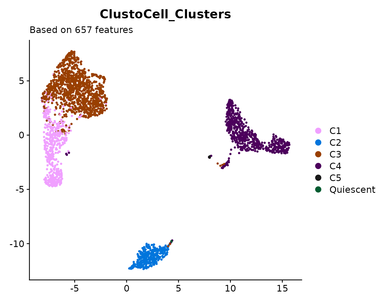
The UMAP shows the major ClustoCell populations identified from the EWCSR-based clustering workflow.


# UMAP visualization of sub-clusters
DimPlot(pbmc3k_so, reduction = "clustoCell_umap", 
        cols = pbmc3k_so$ClustoCell_SubClusters %>% 
          unique() %>% 
          length() %>% 
          DiscretePalette(),
        group.by = "ClustoCell_SubClusters") + 
  labs(x = NULL, y = NULL, 
       subtitle = paste0(
         "Based on ",
         length(pbmc3k_markers$combined_markers),
         " features"
       ))

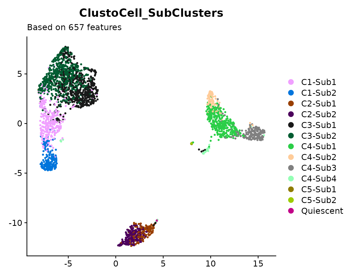
The sub-cluster visualization provides a finer-resolution view of transcriptionally distinct cell states within the major ClustoCell clusters.

Cluster marker evaluation

You can visualize the top markers for your clusters using the markoClustVis function.

You can choose to display positive, negative, or medium markers, or any combination of these. In this example, we show the top positive markers for the major clusters in the pbmc3k dataset.


markoClustVis(obj = pbmc_clustoCell, 
              desired_sets = paste("C", 1:5, sep = ""))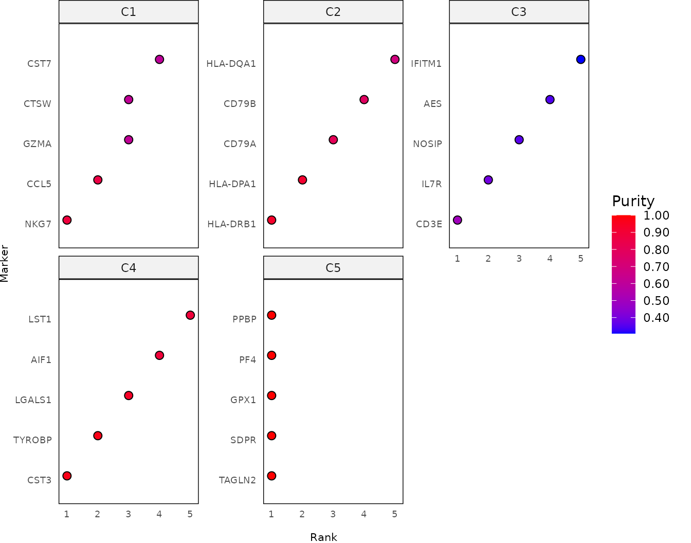

Tip: The cluster and sub-cluster markers are available in pbmc_clustoCell$markers.

Inspecting desired features

In cases where you would like to inspect one or more features (genes) to determine whether they are marker genes for particular clusters or sub-clusters, you can use the featureInspect() function. For example, the following code inspects the genes NKG7 and HLA-DRB1 among the positive markers of the major clusters.


knitr::kable(
  featureInspect(
    clustoCell = pbmc_clustoCell,
    features = c("NKG7", "HLA-DRB1"),
    level = "Major cluster",
    type = "Positive"
  )
)

Feature	Level	Membership	Type	Gini_Score	Purity	Rank
NKG7	Major cluster	C1	Positive	0.1183432	0.8816568	1
HLA-DRB1	Major cluster	C1	Positive	0.9053254	0.0946746	67
HLA-DRB1	Major cluster	C2	Positive	0.0724638	0.9275362	1
HLA-DRB1	Major cluster	C3	Positive	0.9709763	0.0290237	146
HLA-DRB1	Major cluster	C4	Positive	0.3070301	0.6929699	12

As shown above, NKG7 is the top-ranked positive marker of C1 (NK and CD8 T cells), whereas HLA-DRB1 is ranked 1st and 12th among the positive markers of C2 (B cells) and C4 (Mononuclear phagocytes), respectively. Although HLA-DRB1 is also present among the positive markers of two other clusters, it is not sufficiently highly ranked to be particularly informative for annotating those clusters.

The results can also be visualized by setting the plot argument to TRUE.


pbmc_clustoCell_NKG7_HLA_DRB1_plt <-
  featureInspect(
    clustoCell = pbmc_clustoCell,
    features = c("NKG7", "HLA-DRB1"),
    level = "Major cluster",
    type = "Positive",
    plot = TRUE
  )

pbmc_clustoCell_NKG7_HLA_DRB1_plt$plot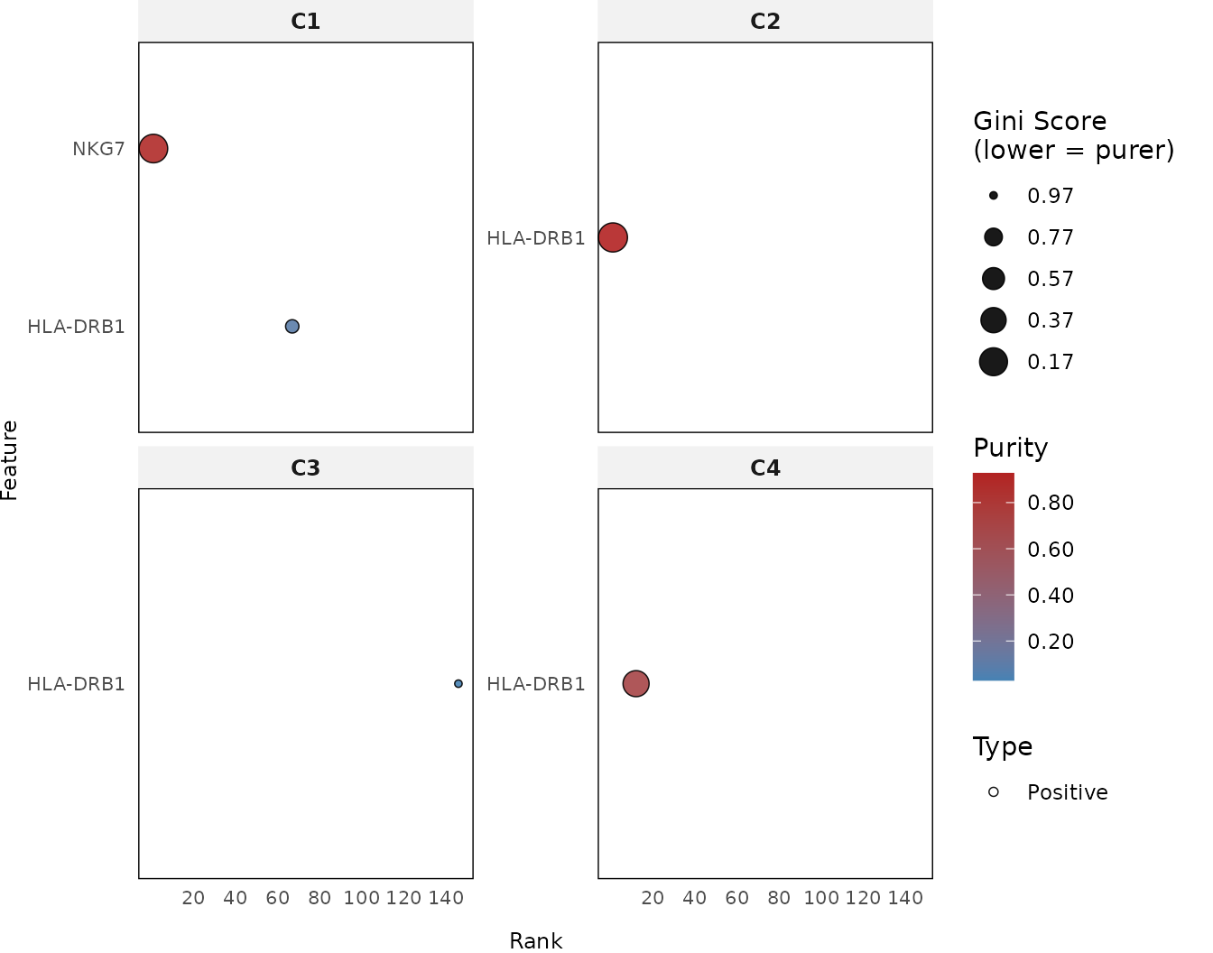

In some cases, your feature(s) of interest may not be identified among the major-cluster or sub-cluster markers. In such situations, you can relax the search by leaving the level and type arguments as NULL (their default values), allowing featureInspect() to search across all available marker collections, including the global feature collections.

For example, if you inspect the general PBMC marker genes CD52, CD53, CD48, and PTPRCAP, while restricting the search to the major-cluster and sub-cluster markers, no matches are returned because these genes are not informative for distinguishing individual cell populations. However, when the level and type arguments are left at their default values, these genes are identified among the globally pure ranked features.

This behaviour is expected because these genes typically exhibit very similar expression patterns across most or all cells in the PBMC dataset. During clustoCell() analysis, such globally uninformative features are automatically detected according to the specified gini_thresh, excluded from the clustering and marker identification procedures to improve sensitivity, and stored in the globally_pure_ranked component of the returned ClustoCell object for future inspection.


knitr::kable(
  featureInspect(
    clustoCell = pbmc_clustoCell,
    features = c("CD52", "CD53", "CD48", "PTPRCAP")
  )
)

Feature	Level	Membership	Type	Gini_Score	Purity	Rank
CD52	Global	Global Features	Pure Ranked	NA	NA	NA
CD53	Global	Global Features	Pure Ranked	NA	NA	NA
CD48	Global	Global Features	Pure Ranked	NA	NA	NA
PTPRCAP	Global	Global Features	Pure Ranked	NA	NA	NA

Tip: Inspecting the global feature collections is particularly useful when analysing datasets composed of a single cell type, where many informative features including canonical marker genes of that cell type are expected to be expressed uniformly across nearly all cells. Such features are typically stored in the globally_pure_ranked or globally_pure_high slot of the ClustoCell object and are not reported as cluster specific markers. See the Working with Single Cell Type Datasets section.

Identifying cluster markers

While clustoCell performs clustering together with marker detection, most clustering methods do not provide markers for each cluster. The markoClust function allows you to identify and rank markers for clusters that you have already defined using other methods.

For example, you may have identified clusters using the Seurat clustering pipeline and want to find the top markers for each cluster to help determine their cell types or subtypes.

Optionally, markoClust can also identify sub-clusters within each cluster while simultaneously detecting their markers (identify_subclusters = TRUE).

In the example below, we first run the standard Seurat clustering pipeline on the pbmc3k dataset, and then use markoClust to identify the top markers for each cluster.


# Running the standard Seurat clustering pipeline
pbmc3k_so <- FindVariableFeatures(pbmc3k_so, 
                                  selection.method = "vst", 
                                  nfeatures = 2000)
pbmc3k_so <- ScaleData(pbmc3k_so)

pbmc3k_so <- RunPCA(pbmc3k_so, npcs = 10, seed.use = 121)

pbmc3k_so <- FindNeighbors(pbmc3k_so, dims = 1:10, 
                           verbose = FALSE)

pbmc3k_so <- FindClusters(pbmc3k_so, resolution = 0.5, 
                          random.seed = 121,
                          verbose = FALSE)

pbmc3k_so <- RunUMAP(pbmc3k_so, dims = 1:10, seed.use = 121)


# UMAP visualization of sub-clusters
DimPlot(pbmc3k_so, reduction = "umap", 
        group.by = "seurat_clusters") + 
  labs(x = NULL, y = NULL)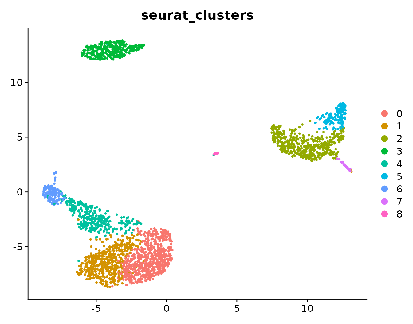


# Running markoClust on Seurat generated clusters (seurat_clusters)
pbmc3k_markoClust <- markoClust(data = pbmc3k_so, 
                                cluster_labels = "seurat_clusters",
                                seed = 121,
                                verbose = FALSE)

Now, let’s visualize the top positive markers identified by markoClust for the Seurat clusters in the pbmc3k dataset.


markoClustVis(obj = pbmc3k_markoClust)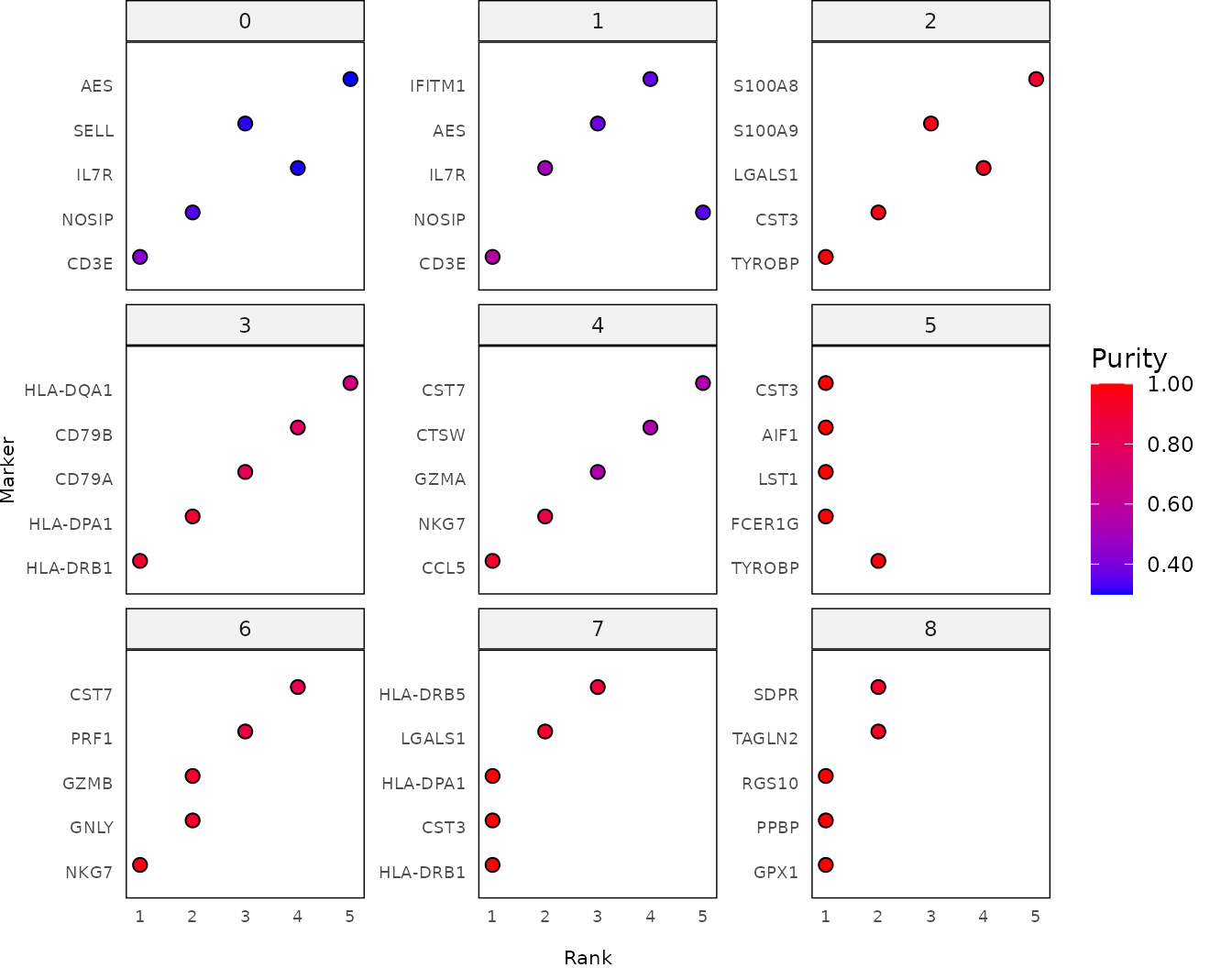

Identifying cell subset markers

In some cases, you may want to find markers for a specific subset of cells, rather than for an entire cluster. The markoCell function is designed for this purpose and can identify markers for both user-defined clusters and selected cell subsets.

More generally, markoCell is useful whenever you want to study the markers and identity of any selected group of cells.

For example, suppose you cluster the same dataset using both ClustoCell and Seurat, and then compare the results. You may notice that most cells from a Seurat cluster match one ClustoCell cluster, but a small subset of cells is assigned differently.


# Visualizing the confusion matrix of ClustoCell and Seurat clusters
table(pbmc3k_so$seurat_clusters, pbmc3k_so$ClustoCell_Clusters) %>% 
  as.data.frame() %>% 
  data.table::setnames(c("Seurat clusters", 
                         "ClustoCell clusters", "Count")) %>% 
  ggplot(aes(x = `ClustoCell clusters`, 
             y = `Seurat clusters`,  
             fill = Count)) +
  geom_point(size = 5, shape = 21) +
  geom_text(aes(label = Count), vjust = -1) +
  scale_fill_gradient(low = "white", 
                       high = scales::muted("#DC0000FF")) +
  theme_minimal()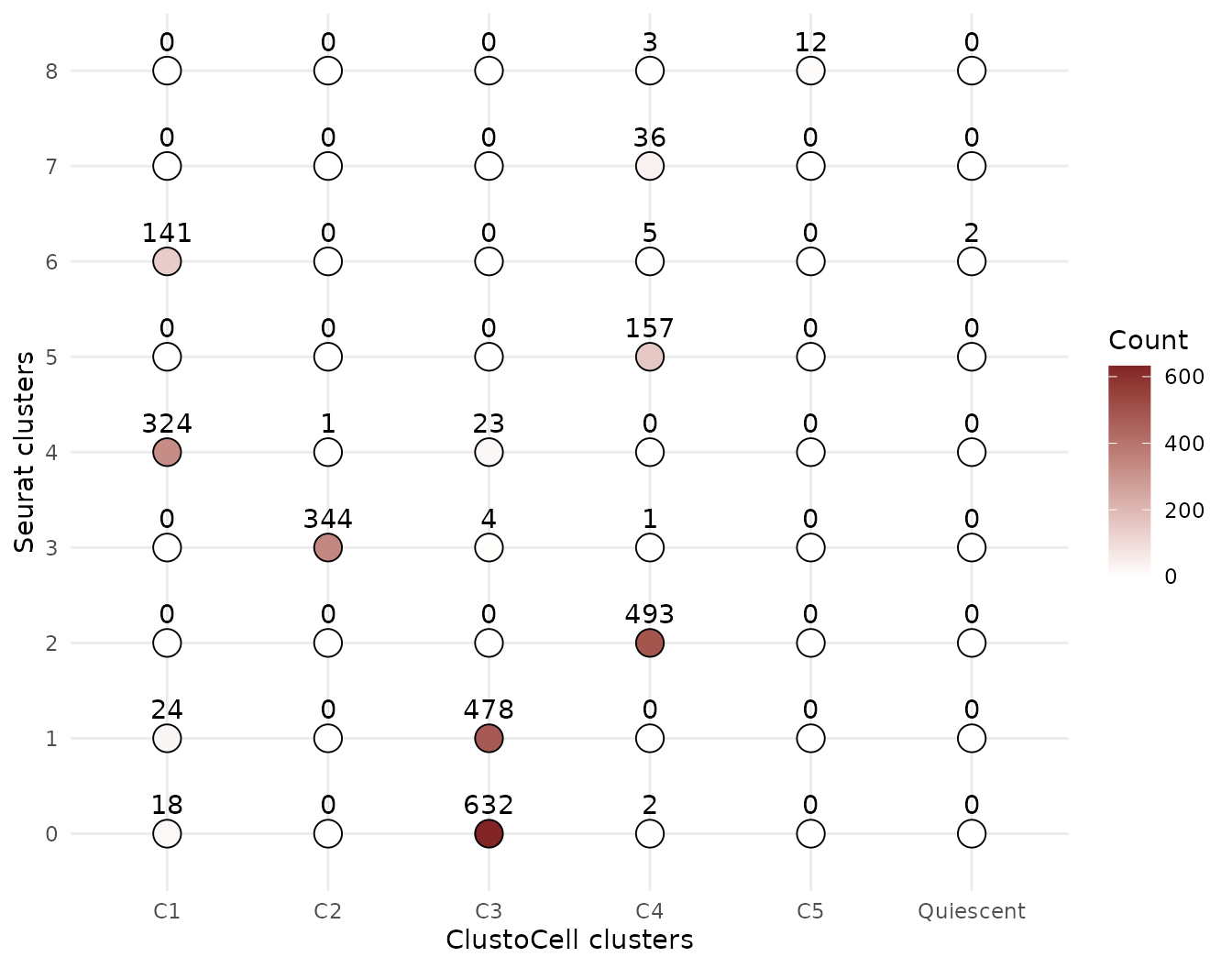

Use case: markoCell() is especially useful for investigating small or ambiguous subsets of cells, such as cells assigned differently by two clustering methods.

In this example, Seurat cluster 1 contains 502 cells and is annotated as memory CD4+ T cells based on its markers. Of these, 478 cells match ClustoCell cluster C3, while 24 cells match ClustoCell cluster C1.

ClustoCell cluster C3 mostly corresponds to Seurat cluster 0/1 (naive/memory CD4+ T cells), whereas ClustoCell cluster C1 mainly corresponds to Seurat cluster 4 (CD8+ cytotoxic T cells). This makes the 24 cells of interest, as they are assigned differently by the two methods.

To better understand their identity, you can use markoCell to identify the key markers for this subset and compare them with the markers of ClustoCell clusters C3 and C1, as well as Seurat clusters 1 and 4.


seurat_1_clustoCell_C1 <- colnames(pbmc3k_so)[
  pbmc3k_so$seurat_clusters == 1 &
    pbmc3k_so$ClustoCell_Clusters == "C1"
]
length(seurat_1_clustoCell_C1)

pbmc3k_1_C1_markoCell <- markoCell(data = pbmc3k_so, 
                                   desired_cells = list(
                                     "s_1_cc_C1" = seurat_1_clustoCell_C1
                                     ), 
                                   seed = 121,
                                   verbose = FALSE)

Now let’s visualize the top markers of this subset of cells.


markoClustVis(obj = pbmc3k_1_C1_markoCell)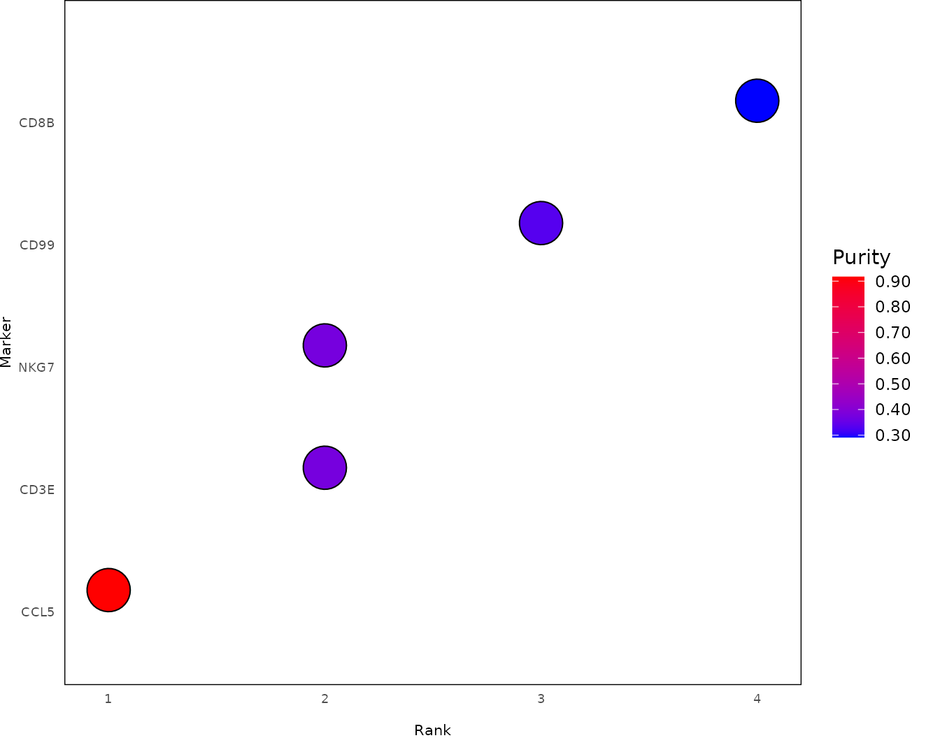

The results show that the top 5 markers of these 24 cells closely match those of Seurat cluster 4 (CD8+ cytotoxic T cells) and ClustoCell cluster C1. This suggests that ClustoCell has more accurately grouped these cells with cytotoxic cells, while Seurat has placed them with memory CD4+ T cells.

Working with Single Cell Type Datasets

There are situations where you may wish to cluster a dataset composed of only a single cell type in order to identify its constituent cell subtypes or cell states and their associated marker genes. For example, upstream enrichment methods such as Fluorescence-Activated Cell Sorting (FACS) physically isolate a specific cell population before sequencing, resulting in a dataset that is highly enriched for the desired cell type. Although ClustoCell is well suited for identifying cell subtypes and states within such datasets, there are several important considerations.

As described in the featureInspect section, when the input dataset consists of a single cell type, many canonical marker genes for that cell type are expected to be expressed uniformly across nearly all cells. Consequently, these features are typically stored in the globally_pure_ranked or globally_pure_high slots of the ClustoCell object. As a result, the top-ranked markers identified for each cluster primarily represent markers that distinguish the corresponding cell subtype or cell state rather than the parent cell type itself. To illustrate this, we subset the PBMC3K dataset to CD8 T cells (C1-Sub1) and rerun clustoCell() on the resulting subset.


# Subsetting the dataset to C1-Sub1 (CD8 cells)
pbmc3k_C1_Sub1_CD8_so <- subset(pbmc3k_so, subset = ClustoCell_SubClusters == "C1-Sub1")

# Running ClustoCell
pbmc3k_C1_Sub1_CD8_clustoCell <- clustoCell(pbmc3k_C1_Sub1_CD8_so, 
                                            identify_subclusters = FALSE,
                                            seed = 121)

Using featureInspect(), we can see that several canonical CD8 T-cell marker genes, including CD3E, GZMA, GZMK, CCL5, and NKG7, are identified as globally pure ranked features in this subset.


knitr::kable(
  featureInspect(
    clustoCell = pbmc3k_C1_Sub1_CD8_clustoCell,
    features = c("CD3E", "GZMA", "GZMK", "CCL5", "NKG7")
  )
)

As shown above, some canonical marker genes of the underlying cell type may not appear among the cluster-specific markers because they are stored in the global feature collections. Therefore, annotation of these subtype/state-focused clusters should make use of the known parent-cell context as well as the cluster-specific markers.

A practical strategy is to construct a marker panel by combining canonical markers of the input cell type (obtained from the literature or by inspecting the global feature collections) with the top cluster-specific markers (e.g. the top 10–15 positive markers). The resulting panel can be interpreted manually, queried against the Marker DB with typoClust(mode = "markerDB"), or supplied to ceLLMarkup() for LLM-assisted interpretation.

Tip: For pre-enriched single-cell-type datasets, explicitly provide the known biological context whenever possible. See the custom marker panel, ceLLMarkup(), and typoPrompt() sections for complementary annotation strategies.


pbmc3k_C1_Sub1_CD8_clustoCell_C1_typoClust <- 
  typoClust(
    desired_pos_markers = list(
      my_panel = c(
        "CD3E", "GZMA", "GZMK", "CCL5", "NKG7",
        pbmc3k_C1_Sub1_CD8_clustoCell$markers$major_clusters$cluster_specific$positive_markers$C1$Feature[1:5]
      )
    ),
    tissue = "Blood",
    mode = "markerDB",
    species = "human",
    verbose = FALSE
  )

Let’s look at the top-ranked predicted cell type (or cell state).


knitr::kable(
  pbmc3k_C1_Sub1_CD8_clustoCell_C1_typoClust$cell_types$my_panel[
    1, c("Tissue", "Condition", "CellType", "Combined_Score", "Rank")
  ]
)

Tissue	Condition	CellType	Combined_Score	Rank
Blood	Healthy	CD8+ Alpha-Beta T Cell	6042.57	1

As expected, the cluster is annotated as CD8+ Alpha-Beta T Cell.

Note: If you are unsure whether your dataset contains multiple cell types or represents a single cell type, inspect both the top cluster-specific markers and the canonical marker genes that may have been assigned to the global feature collections. For example, if one cluster is characterised by canonical NK/CD8 T-cell markers such as NKG7, CCL5, GZMA, CTSW, CST7, and GNLY, whereas another cluster is characterised by canonical B-cell markers such as HLA-DRB1, HLA-DPA1, CD79A, CD79B, HLA-DQA1, and HLA-DQB1, then your dataset clearly contains multiple cell types rather than a single homogeneous cell population.

Assessing purity of markers

In some cases, you may have a specific marker in mind and want to check how purely it is expressed in a particular cluster or subset of cells. The markerPurity function allows you to do this quickly.

It uses the EWCSR framework and Gini coefficient to measure purity, defined as the proportion of cells in the selected group that show high expression of the marker.

For example, you can use markerPurity to examine how purely the gene NKG7 is expressed in Seurat cluster 6.


pbmc3k_6_NKG7_markerPurity <-
  markerPurity(data = pbmc3k_so, 
               desired_markers = "NKG7", 
               cluster_labels = "seurat_clusters", 
               desired_clusters = "6",
               seed = 121,
               verbose = FALSE)


knitr::kable(pbmc3k_6_NKG7_markerPurity$within_clusters$positive_markers$`6`)

Feature	Gini_Score	Purity	Rank
NKG7	0.0337838	0.9662162	1

Cell type annotation

CelliVerse provides several complementary routes for annotating clusters, sub-clusters, or selected cell subsets. You can use the curated CelliVerse Marker DB, connect directly to a local or cloud LLM, or generate a structured prompt that can be pasted into a chatbot of your choice.

The CelliVerse Marker DB is a curated collection of positive and negative marker genes for human and mouse, stored in a sparse matrix format. It combines information from several major resources, including Cell Marker Accordion, CellMarker2, DISCO, PanglaoDB, ScTypeDB, and singleCellBase.

Curated database

`typoClust(mode = “markerDB”)`

Matches positive and/or negative markers against the CelliVerse Marker DB. This route does not require an LLM or API key.

Direct LLM

`typoClust(mode = “ceLLMarkup”)`

Uses markers from ClustoCell/MarkoCell objects or supplied panels and delegates annotation to ceLLMarkup().

Direct LLM

`ceLLMarkup()`

Annotates marker tables, Seurat FindAllMarkers() output, or marker panels using a supported local or cloud model.

Portable prompt

`typoPrompt()`

Builds a copy-and-paste-ready annotation prompt from a ClustoCell or MarkoCell object without contacting an LLM.

Important: Automatic annotations should be treated as evidence-supported suggestions rather than definitive labels, particularly when distinguishing closely related cell subtypes or transient cell states. The cluster-specific markers identified by ClustoCell or MarkoCell should remain central to biological interpretation, and annotations should be checked against marker biology, experimental context, and prior knowledge.

Major-cluster inheritance: Both typoClust() and ceLLMarkup() use inherit_major_clusters = TRUE by default when a major cluster and its sub-clusters are available. The major cluster is annotated first, and each sub-cluster is then interpreted using its own markers within the biological identity of that parent. This can improve hierarchical consistency, but the parent label should be treated as a useful prior rather than an absolute constraint. If a major cluster is broad, mixed, or ambiguously annotated, inheritance can limit recovery of biologically distinct subtypes or states. In such cases, compare the results with inherit_major_clusters = FALSE.

Marker DB annotation with `typoClust()`

typoClust() can annotate marker results stored in one or more ClustoCell or MarkoCell objects, or it can work directly from user-supplied positive and/or negative marker panels.

Positive markers support a candidate cell identity.
Negative markers provide exclusionary evidence and can help distinguish closely related identities.

When mode = "markerDB", tissue and condition can be used to restrict the marker-database search to biologically relevant contexts. When objects are supplied, thresh_mode and thresh control how many top-ranked markers are used for each set.

Controlling major-cluster inheritance

By default, inherit_major_clusters = TRUE. When a ClustoCell or MarkoCell object contains both major clusters and sub-clusters, typoClust() first annotates the parent major cluster from the major cluster’s own markers and then annotates each sub-cluster from the sub-cluster’s own markers, while using the parent identity to guide the interpretation. A parent that is required for this step is annotated and returned even if it was not explicitly included in desired_sets. The inheritance used for each sub-cluster is also recorded in metadata$inheritance.

How the parent identity is used depends on the annotation mode:

With mode = "markerDB", the Marker DB is restricted to the parent identity and cell types whose names represent varieties of that identity. The inherit_score_ratio argument controls whether near-tied parent candidates are also admitted. Its default is 0.5. For example, a value of 1 uses only the rank-1 parent label, whereas 0.6 also admits any candidate whose score is at least 60% of the rank-1 score. Lower values therefore allow more plausible parent identities and make the inheritance less restrictive. inherit_score_ratio is used only for Marker DB annotation.
With mode = "ceLLMarkup", the LLM is told the inferred parent identity and is asked which subtype, differentiation state, activation state, or functional state of that parent best matches each sub-cluster. inherit_score_ratio does not apply in this mode.

You can disable the hierarchy at any time with inherit_major_clusters = FALSE. In that case, clusters and sub-clusters are annotated independently.

PBMC3K example and why this matters: In the PBMC3K analysis used throughout this vignette, major cluster C1 groups CD8+ T cells and NK cells, while sub-clustering separates the CD8+ T-cell population from the NK-cell population. Both lineages arise from common lymphoid progenitors and share strong cytotoxic transcriptional programs, so their grouping within a broader major cluster is biologically plausible. However, the Marker DB does not contain a single combined label such as “CD8+ T and NK Cell”. The major cluster must therefore be assigned to the closest available identities. In this dataset, the top candidates for C1 are NK Cell and CD8+ Alpha-Beta T Cell, with the second candidate scoring approximately 65% of the first. If only the rank-1 parent were inherited, for example with inherit_score_ratio = 1, the CD8+ T-cell sub-cluster could be restricted to NK-related labels even though its own markers support a T-cell identity. At the default inherit_score_ratio = 0.5, both parent candidates are admitted, which preserves a broader and more appropriate vocabulary for the C1 sub-clusters.

Practical recommendation: Major-cluster inheritance is most useful when the parent identity is biologically coherent and confidently annotated. For broad or mixed major clusters, or whenever the parent annotation is uncertain, it is worth running annotation once with inheritance enabled and once with inherit_major_clusters = FALSE, then comparing the resulting labels with the sub-cluster-specific markers and biological context. This is especially important for fine cell-type and cell-state annotation, where an incorrect or overly broad parent label can otherwise propagate to all of its sub-clusters.

For example, the C1 hierarchy can be compared directly using:

# Hierarchical annotation using the defaults
pbmc_C1_inherited <- typoClust(
  objects = list(pbmc_clustoCell),
  desired_sets = c("C1", "C1-Sub1", "C1-Sub2"),
  tissue = "Blood",
  condition = "Healthy",
  mode = "markerDB",
  inherit_major_clusters = TRUE,
  inherit_score_ratio = 0.5,
  species = "human",
  verbose = FALSE
)

# Annotate the same sets independently
pbmc_C1_independent <- typoClust(
  objects = list(pbmc_clustoCell),
  desired_sets = c("C1", "C1-Sub1", "C1-Sub2"),
  tissue = "Blood",
  condition = "Healthy",
  mode = "markerDB",
  inherit_major_clusters = FALSE,
  species = "human",
  verbose = FALSE
)

You can inspect the available tissue and disease-condition labels as shown below.

data("tissueCondition_types", package = "celliverse")

# Or:
# tissueCondition_types <- celliverse::tissueCondition_types

head(tissueCondition_types$human$diseased_tissueCondition)

Tissue	Condition
Adipose Tissue	Breast Cancer
Adrenal Gland	Neuroblastoma
Adrenal Gland	Adrenal Neuroblastoma
Airway	Lung Adenocarcinoma
Alveolus of Lung	Non Small Cell Lung Cancer
Amniotic Fluid	Amniotic Fluid

In the example below, we annotate the five major ClustoCell clusters identified in the PBMC3K dataset using the CelliVerse Marker DB.

clustoCell_pbmc_typoClust <- typoClust(
  objects = list(pbmc_clustoCell),
  desired_sets = paste0("C", 1:5),
  tissue = "Blood",
  mode = "markerDB",
  species = "human",
  verbose = FALSE
)

Let’s have a look at the top candidates for C1.

head(
  clustoCell_pbmc_typoClust$cell_types$C1[
    , c("Tissue", "Condition", "CellType", "Combined_Score", "Rank")
  ]
)

Tissue	Condition	CellType	Combined_Score	Rank
Blood	Healthy	NK Cell	9043.118	1
Blood	Healthy	T Cell	5146.334	2
Blood	Healthy	CD8+ Alpha-Beta T Cell	5038.638	3
Blood	Healthy	NKT Cell	3558.503	4
Blood	Healthy	CD8+ Effector T Cell	3117.143	5
Blood	Healthy	Gamma-Delta T Cell	2907.157	6

Cell type annotation based on a custom marker panel

Custom marker panels are useful when you have marker genes for a selected cell population but do not have a ClustoCell or MarkoCell object for that population.

For example, suppose the genes NKG7, CCL5, GZMA, CTSW, CST7, GNLY, CD99, GZMB, and PRF1 define a cell subset of interest. You can query this panel against the Marker DB as follows.

my_panel_typoClust <- typoClust(
  desired_pos_markers = list(
    my_panel = c(
      "NKG7", "CCL5", "GZMA", "CTSW",
      "CST7", "GNLY", "CD99", "GZMB", "PRF1"
    )
  ),
  tissue = "Blood",
  mode = "markerDB",
  species = "human",
  verbose = FALSE
)

head(
  my_panel_typoClust$cell_types$my_panel[
    , c("Tissue", "Condition", "CellType", "Combined_Score", "Rank")
  ]
)

Tissue	Condition	CellType	Combined_Score	Rank
Blood	Healthy	NK Cell	13115.828	1
Blood	Healthy	CD8+ Alpha-Beta T Cell	10024.184	2
Blood	Healthy	NKT Cell	6492.006	3
Blood	Healthy	T Cell	6338.380	4
Blood	Healthy	CD8+ Effector T Cell	5386.366	5
Blood	Healthy	CD4+ Alpha-Beta Cytotoxic T Cell	4305.613	6

Choosing between “n” and “rank”: With thresh_mode = “n”, exactly the first thresh rows are selected when available. With thresh_mode = “rank”, all markers up to the requested rank are retained, including markers tied at the cutoff rank.

LLM annotation through `typoClust()`

Set mode = "ceLLMarkup" when you want typoClust() to use an LLM instead of the Marker DB. This keeps the familiar ClustoCell/MarkoCell workflow while passing the selected marker panels to ceLLMarkup() for model-based annotation.

Supported providers include Ollama and LM Studio for local models, as well as OpenAI, Anthropic, Gemini, DeepSeek, Groq, OpenRouter, and Cerebras for cloud models.

The following example uses a local Ollama model. It is not run while building the vignette because it requires a running model server and model inference.

clustoCell_pbmc_typoClust_llm <- typoClust(
  objects = list(pbmc_clustoCell),
  desired_sets = paste0("C", 1:5),
  tissue = "Blood",
  condition = "Healthy",
  mode = "ceLLMarkup",
  species = "human",
  llm_provider = "ollama",
  llm_model = "qwen3:8b",
  llm_top_k = 3,
  verbose = FALSE
)

For a cloud provider, specify the corresponding provider and model. API keys can be supplied through llm_api_key, but for reproducible and secure workflows it is generally preferable to use the provider’s standard environment variable rather than hard-coding a key in an R script.

Inheritance in LLM mode: inherit_major_clusters = TRUE also applies when typoClust(mode = “ceLLMarkup”) is used. The LLM first annotates the major cluster and then receives that parent identity when interpreting its sub-clusters. Because the parent call can depend on the model and on the selected marker set, a broad or mixed major cluster may sometimes lean toward one of its constituent lineages. In that situation, inheritance can make the downstream subtype/state calls too restrictive. If the sub-cluster markers suggest a different lineage or a more appropriate state, compare with inherit_major_clusters = FALSE. The inherit_score_ratio argument is specific to mode = “markerDB” and is ignored for LLM annotation.

LLM reproducibility and privacy: LLM annotations can vary across model versions, providers, and sampling settings. Record the provider and model used for important analyses. When using a cloud provider, marker and biological-context information included in the request is sent to that provider. Use Ollama or LM Studio when a fully local annotation workflow is required.

Direct LLM annotation with `ceLLMarkup()`

ceLLMarkup() can also be called directly when you want LLM-based annotation without going through typoClust(). Exactly one of the following input modes is supplied:

marker_set_list: a named list of marker data frames;
seuratClusters: a data frame returned by Seurat’s FindAllMarkers(); or
panels: positive marker panels, optionally accompanied by negative marker panels.

This makes ceLLMarkup() useful when your markers were generated outside CelliVerse or when you want finer control over LLM-specific settings such as temperature, n_markers, and max_retries.

ceLLMarkup() also uses inherit_major_clusters = TRUE by default. When the supplied set names contain both a parent and its sub-clusters, for example C1, C1-Sub1, and C1-Sub2, the function identifies the major cluster first and then issues a separate second-stage annotation for the sub-clusters of each parent. The model is explicitly asked to interpret those sets as subtypes or states of that parent using the sub-cluster-specific markers. If only sub-clusters are supplied without their parent, there is no parent identity to inherit and they are annotated in the ordinary independent manner. Set inherit_major_clusters = FALSE when you want all supplied sets to be annotated independently.

For example, the following marker panels can be annotated with a local Ollama model.

pbmc_llm_annotations <- ceLLMarkup(
  panels = list(
    C1 = c("NKG7", "GNLY", "GZMA", "CST7", "PRF1"),
    C2 = c("CD79A", "CD79B", "MS4A1", "CD74", "HLA-DRA")
  ),
  sample_source = "human peripheral blood",
  feature_type = "gene",
  tissue = "Blood",
  condition = "Healthy",
  species = "human",
  provider = "ollama",
  model = "qwen3:8b",
  temperature = 0.2,
  top_k = 3,
  n_markers = 25,
  verbose = FALSE
)

The returned object is TypoClust-compatible, allowing LLM-based annotations to fit naturally into downstream CelliVerse annotation workflows.

When should I call ceLLMarkup() directly? Use typoClust(mode = “ceLLMarkup”) when your markers are already stored in ClustoCell or MarkoCell objects and you want the usual typoClust() interface. Use ceLLMarkup() directly when starting from Seurat marker results, standalone marker tables, or custom panels, or when you need its LLM-specific controls.

Generate a portable LLM prompt with `typoPrompt()`

typoPrompt() provides a third LLM-assisted route without connecting R to a model provider. It extracts marker information from a ClustoCell or MarkoCell object, adds the available biological context, and constructs a structured prompt for cell type, subtype, or cell-state annotation.

This is useful when you prefer to paste the prompt into an existing ChatGPT, Claude, Gemini, or other chatbot session, or when you want to inspect exactly what will be supplied to the model before submitting it.

The returned TypoPrompt object provides:

a formatted and a raw prompt view;
collapsible sections for long prompts;
light and dark appearance;
one-click copying;
TXT and HTML downloads;
printing to PDF; and
direct plain-text access through cat() or as.character().

Unlike ceLLMarkup(), generating the prompt itself does not require an API key, local model, or model server.

For the same pbmc_clustoCell object used throughout this vignette, we can generate a prompt for the five major clusters:

pbmc_typoPrompt <- typoPrompt(
  object = pbmc_clustoCell,
  desired_sets = paste0("C", 1:5),
  sample_source = "human peripheral blood",
  feature_type = "gene",
  species = "human",
  tissue = "Blood",
  condition = "Healthy",
  use_neg_markers = TRUE,
  thresh_mode = "n",
  thresh = 20,
  top_k = 3,
  verbose = FALSE
)

When TypoPrompt is printed interactively, its full HTML interface opens in the RStudio Viewer, or in the default browser when the Viewer is unavailable. The vignette embeds that same HTML renderer below so that the prompt can be inspected without leaving this page.

Live vignette previewPBMC3K cell-type annotation prompt

Scroll inside the preview to inspect the complete prompt

The underlying prompt is still an ordinary character-like object and can be inspected directly:

cat(pbmc_typoPrompt)
as.character(pbmc_typoPrompt)

It can also be exported programmatically:

saveTypoPrompt(
  pbmc_typoPrompt,
  file = "pbmc_cell_annotation_prompt.txt",
  format = "txt"
)

saveTypoPrompt(
  pbmc_typoPrompt,
  file = "pbmc_cell_annotation_prompt.html",
  format = "html"
)

ClustoCell hierarchy awareness: When a prompt contains a major ClustoCell cluster together with its sub-clusters, typoPrompt() adds instructions describing that hierarchy. The LLM is asked to establish the parent identity first and then interpret sub-clusters as more specific subtypes or states where supported by the markers.

Adding cell type annotations to the dataset

After obtaining a TypoClust-compatible annotation object from typoClust() or ceLLMarkup(), you can add the inferred cell type annotations back to your Seurat or SingleCellExperiment object using addTypoData().

The cell type labels are added to the metadata as new columns, based on the specified clusters or cell subsets. You can include multiple ranked cell type predictions, and optionally refine them to more specific labels by adjusting the rank_thresh and refine_thresh arguments.

In the example below, we add the cell type annotations for the 5 major ClustoCell clusters (stored in the clustoCell_pbmc_typoClust object) back to the PBMC Seurat object.


pbmc3k_so <- addTypoData(obj = pbmc3k_so, 
                         typoClust = clustoCell_pbmc_typoClust,
                         clusters = c("ClustoCell_Clusters"))

Visualizing cell type annotations

To visualize cell type annotation results stored in a TypoClust-compatible object, you can use typoClustVis().

In the example below, we display the Marker DB annotations for the five major ClustoCell clusters in the PBMC3K dataset. The same visualization workflow can be used for compatible LLM-based annotation results.


typoClustVis(clustoCell_pbmc_typoClust, 
             order_by = "Cluster")
#> ℹ Since `desired_sets` is NULL, all clusters and cell subsets will be visualized!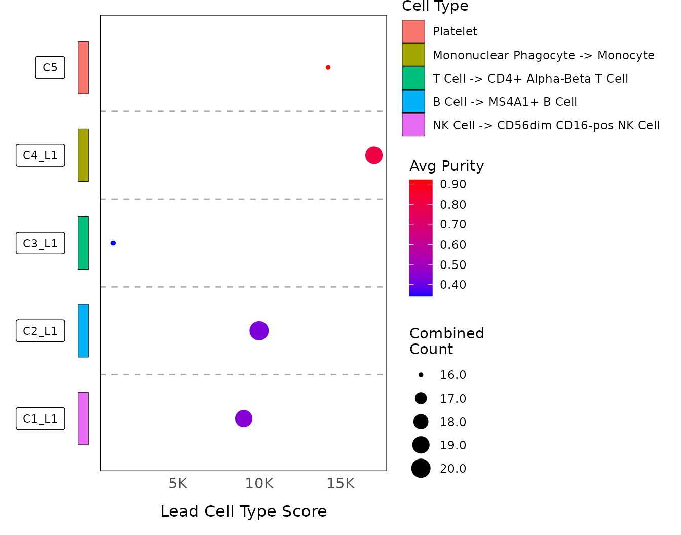

Visualizing signature expressions

In some cases, you may have predefined sets of marker genes (signatures) and want to see how strongly each cluster in your dataset expresses these signatures. The signatureDotHeatmap function can be used to visualize this as a dot heatmap.

For example, suppose you have five gene signatures representing different cell types:

CD4+ T cells (CD4 T): IL7R, SELL, NOSIP, AES, RARRES3
B cells (B): CD79A, CD79B, MS4A1, TCL1A, HLA-DRB1
Cytotoxic lymphocytes (CL): NKG7, GNLY, GZMA, CST7, PRF1
Mononuclear phagocytes (MNP): S100A8, S100A9, FCN1, AIF1, LST1
Platelets (PLT): PPBP, PF4, SDPR, GP9, GPX1

First, create a row_data data frame that defines these signatures, as shown below.


pbmc_row_data <- 
  data.frame(
    Features = c(
      "IL7R", "SELL", "NOSIP", "AES", "RARRES3",
      "CD79A", "CD79B", "MS4A1", "TCL1A", "HLA-DRB1",
      "NKG7", "GNLY", "GZMA", "CST7", "PRF1",
      "S100A8", "S100A9", "FCN1", "AIF1", "LST1",
      "PPBP", "PF4", "SDPR", "GP9", "GPX1"
    ),
    Signature = rep(c(
      "CD4 T",
      "B",
      "CL",
      "MNP",
      "PLT"
    ), each = 5)
  )


head(pbmc_row_data)

Features	Signature
IL7R	CD4 T
SELL	CD4 T
NOSIP	CD4 T
AES	CD4 T
RARRES3	CD4 T
CD79A	B

Then, you can use signatureDotHeatmap to visualize the overall expression of these signatures across the five major ClustoCell clusters in the pbmc3k dataset.


signatureDotHeatmap(
  seurat_obj = pbmc3k_so,
  cluster_col = "ClustoCell_Clusters",
  row_data = pbmc_row_data, 
  features_col = "Features", 
  signature_col = "Signature")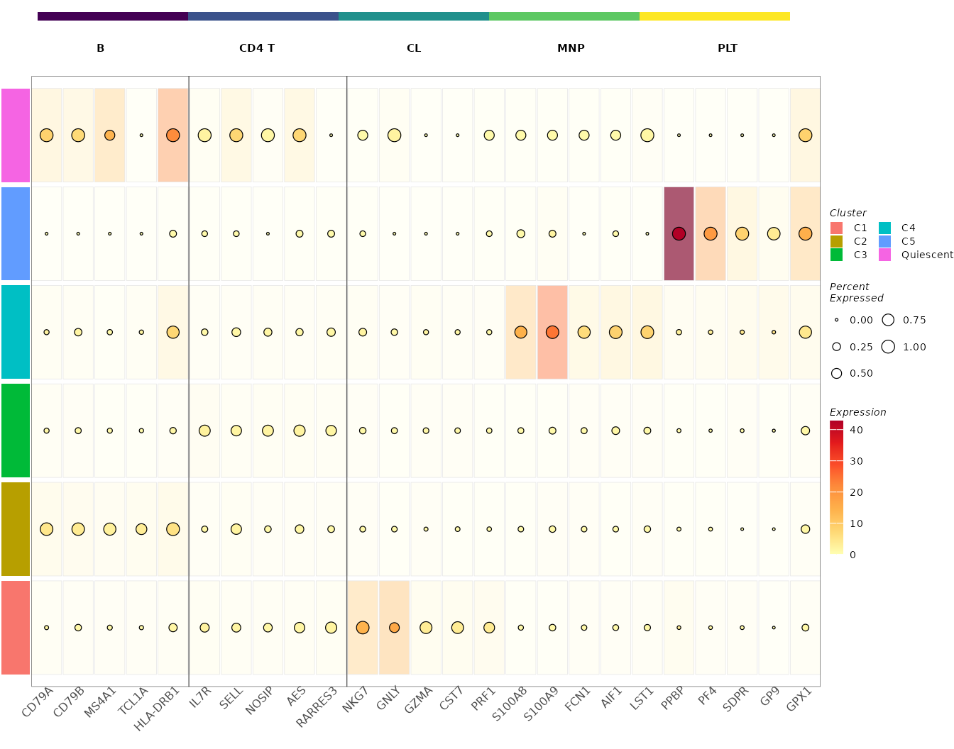

Running ClustoCell on large datasets

Large dataset recommendation: For datasets with hundreds of thousands to millions of cells, consider using sketching or the decoupled sketching plus label-transfer workflow. This can substantially reduce memory use and runtime while preserving the ability to annotate the full dataset.

ClustoCell can take longer to run on large single-cell datasets with hundreds of thousands or millions of cells. If you run into memory or performance issues, or simply want to speed up the analysis, you can enable the sketching option by setting sketch = TRUE.

Sketching is intended as a scalability strategy. It reduces runtime and memory requirements by clustering a representative subset of cells, while label transfer allows the final annotations to be mapped back to the complete dataset.

When sketching is enabled, ClustoCell (and markoClust) first performs preprocessing and feature filtration on the full dataset. It then creates a smaller sketched dataset, performs clustering and sub-clustering on this subset, and finally transfers the cluster labels back to the full dataset using an internal label transfer step. You can control the size of the sketched dataset using the sketch_ncells argument (default is 5000).

In the example below, we run ClustoCell with sketching enabled on the pbmc3k dataset (for simplicity), but the same approach applies to datasets of any size.


pbmc_clustoCell_withSketch <- clustoCell(
  data = pbmc3k_so, 
  sketch = TRUE, 
  sketch_ncells = 1500, 
  identify_subclusters = FALSE,
  seed = 121,
  verbose = FALSE
)

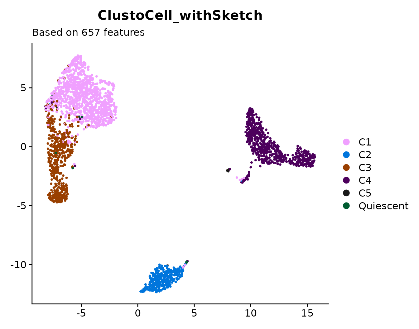
After running ClustoCell, you can add the cluster labels back to the Seurat object and visualize them.


pbmc3k_so <- addClustoData(
  obj         = pbmc3k_so,
  clustoCell  = pbmc_clustoCell_withSketch, 
  major_cluster_name = "ClustoCell_withSketch", 
  add_sub_clusters = FALSE
)


DimPlot(pbmc3k_so, reduction = "clustoCell_umap", 
        cols = pbmc3k_so$ClustoCell_withSketch %>% 
          unique() %>% 
          length() %>% 
          DiscretePalette(),
        group.by = "ClustoCell_withSketch") + 
  labs(x = NULL, y = NULL,
       subtitle = paste0(
         "Based on ",
         length(pbmc3k_markers$combined_markers),
         " features"
       ))

You can also compare the results by looking at a confusion matrix between:

ClustoCell run on the full dataset, and
ClustoCell run with sketching and label transfer


table(pbmc3k_so$ClustoCell_withSketch, pbmc3k_so$ClustoCell_Clusters) %>% 
  as.data.frame() %>% 
  data.table::setnames(c("ClustoCell with sketch", 
                         "ClustoCell without sketch", "Count")) %>% 
  ggplot(aes(x = `ClustoCell without sketch`, 
             y = `ClustoCell with sketch`,  
             fill = Count)) +
  geom_point(size = 5, shape = 21) +
  geom_text(aes(label = Count), vjust = -1) +
  scale_fill_gradient(low = "white", 
                       high = scales::muted("#DC0000FF")) +
  theme_minimal()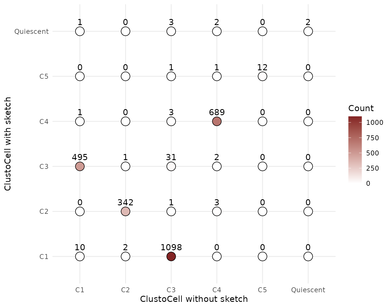

In this example, the results show near-perfect agreement, indicating that sketching provides similar results while being much faster.

Sub-clustering with sketching

When identify_subclusters = TRUE, ClustoCell also detects sub-clusters. If you use this together with sketch = TRUE, clustering and sub-clustering are both performed on the sketched data, and the labels are then transferred back to the full dataset.

There is also an optional argument, refine_transferred_subClusters, which changes how sub-clusters are assigned:

If refine_transferred_subClusters = FALSE (default), sub-cluster labels are directly transferred from the sketched data.
If refine_transferred_subClusters = TRUE, ClustoCell first transfers major cluster labels to the full dataset, and then runs sub-cluster detection separately within each major cluster using the full data.

This refinement step can take more time, but it often improves the quality of sub-clusters. Since sub-clustering is performed within each major cluster (which is much smaller than the full dataset), it is still much faster than running ClustoCell on the entire dataset without sketching.

In the example below, we demonstrate this sub-cluster refinement approach on the pbmc3k dataset.


pbmc_clustoCell_withSketch <- clustoCell(
  data = pbmc3k_so, 
  sketch = TRUE, 
  sketch_ncells = 1500, 
  identify_subclusters = TRUE, 
  refine_transferred_subClusters = TRUE,
  seed = 121,
  verbose = FALSE
)

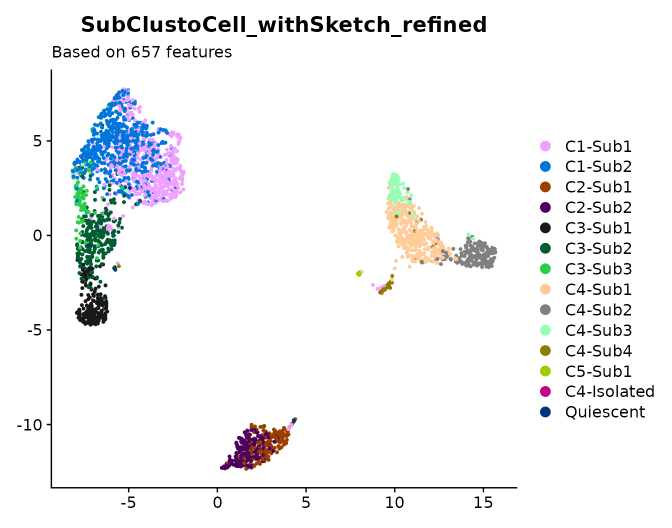
Afterwards, we again add the cluster labels back to the Seurat object and visualize them.


pbmc3k_so <- addClustoData(
  obj         = pbmc3k_so,
  clustoCell  = pbmc_clustoCell_withSketch, 
  sub_cluster_name = "SubClustoCell_withSketch_refined", 
  add_major_clusters = FALSE
)


DimPlot(pbmc3k_so, reduction = "clustoCell_umap", 
        cols = pbmc3k_so$SubClustoCell_withSketch_refined %>% 
          unique() %>% 
          length() %>% 
          DiscretePalette(),
        group.by = "SubClustoCell_withSketch_refined") + 
  labs(x = NULL, y = NULL,
       subtitle = paste0(
         "Based on ",
         length(pbmc3k_markers$combined_markers),
         " features"
       ))

Finally, we compare the results using a confusion matrix between:

Sub-clusters from the full dataset, and
Refined sub-clusters obtained with sketching


table(pbmc3k_so$SubClustoCell_withSketch_refined, pbmc3k_so$ClustoCell_SubClusters) %>% 
  as.data.frame() %>% 
  data.table::setnames(c("Refined SubClustoCell with sketch", 
                         "SubClustoCell without sketch", "Count")) %>% 
  ggplot(aes(x = `SubClustoCell without sketch`, 
             y = `Refined SubClustoCell with sketch`,  
             fill = Count)) +
  geom_point(size = 5, shape = 21) +
  geom_text(aes(label = Count), vjust = -1) +
  scale_fill_gradient(low = "white", 
                       high = scales::muted("#DC0000FF")) +
  theme_minimal() +
  theme(axis.text.x = element_text(angle = 25, vjust = 0.8))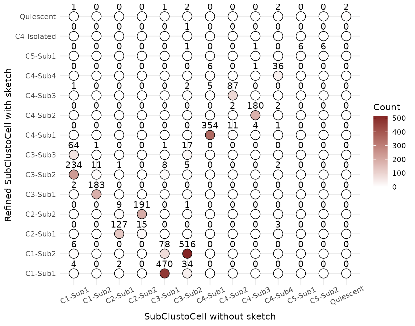

The results show very high agreement, indicating that sketching with refinement maintains accuracy while improving performance for detecting sub-clusters.

Decoupling sketching and label transfer

When to decouple: Use the built-in sketch = TRUE workflow for moderate-to-large datasets. For very large datasets or limited computational resources, first create a sketched object externally, run clustoCell() only on the sketch, and then transfer labels back to the full dataset.

As mentioned earlier, when running clustoCell or markoClust with sketch = TRUE, the functions still perform preprocessing and feature filtration on the full dataset before sketching. For very large datasets, this initial step can still be slow and resource-intensive.

In such cases, it is recommended to separate (decouple) the sketching and label transfer steps.

In this approach:

First, create a smaller dataset by sketching the full data (for example, using Seurat’s SketchData function).
Then, run clustoCell on the sketched dataset only. This avoids preprocessing and feature selection on the full dataset.
Finally, transfer the cluster labels from the sketched data back to the full dataset using clustoCell_TransferLabel and addClustoData functions.

The clustoCell_TransferLabel function returns an updated ClustoCell object including cluster labels for the full dataset.

This strategy is especially useful when working with very large datasets or limited computational resources.

Expression-based label transfer: The “seurat-project” and “seurat-knn” methods operate on the original expression matrix rather than the EWCSR representation. The input expression data may consist of raw counts, log-normalized values, or SCTransform-normalized data, provided that both the sketched and full datasets use the same normalization strategy.

In the example below, we demonstrate this approach using the pbmc3k dataset and perform label transfer using the "seurat-project" method.

Verify that sketching has reduced the dataset: Before applying SketchData(), it is recommended to run NormalizeData() and FindVariableFeatures() on the input assay. Depending on the structure and preprocessing state of the input assay, particularly when normalized data or variable features are unavailable, sketching may not be performed as expected. In such cases, the newly generated sketch assay may contain the same number of cells as the original assay. Always inspect the number of cells in the sketch assay before running clustoCell().


# Set the original assay as the active assay
DefaultAssay(pbmc3k_so) <- "RNA"

# Normalize the input assay and identify variable features
# before applying sketching
pbmc3k_so <- NormalizeData(
  object = pbmc3k_so,
  assay = "RNA",
  verbose = FALSE
)

pbmc3k_so <- FindVariableFeatures(
  object = pbmc3k_so,
  assay = "RNA",
  verbose = FALSE
)

# Record the number of cells in the full dataset
n_full_cells <- length(Cells(pbmc3k_so))

# Sketching the data
pbmc3k_so <- SketchData(
  object = pbmc3k_so,
  assay = "RNA",
  ncells = 1500,
  method = "Uniform",
  sketched.assay = "sketch",
  seed = 121,
  verbose = FALSE
)

# Verify that the sketch contains fewer cells than the
# original dataset
n_sketch_cells <- length(Cells(pbmc3k_so[["sketch"]]))

message(
  "Full dataset: ", n_full_cells, " cells; ",
  "sketched assay: ", n_sketch_cells, " cells."
)

if (n_sketch_cells >= n_full_cells) {
  stop(
    "Sketching did not reduce the number of cells. ",
    "Check that the input assay contains normalized data and ",
    "variable features before continuing."
  )
}

# Running clustoCell on the verified sketched assay
sketched_pbmc_clustoCell <- clustoCell(
  data = pbmc3k_so,
  assay = "sketch",
  seed = 121,
  verbose = FALSE
)

Note that in the SketchData() function we set the sketched.assay argument to “sketch”, and when running clustoCell() we set the assay argument to the same newly generated assay, “sketch”. However, during the label transfer step below using clustoCell_TransferLabel(), the full-data assay must be provided. Therefore, we set the assay argument to the original assay, “RNA”.


# Converting the ClustoCell object to full dataset mode
sketched_pbmc_clustoCell <- 
  clustoCell_TransferLabel(
    clustoCell = sketched_pbmc_clustoCell, 
    query_expr_mat = pbmc3k_so, 
    assay = "RNA",
    method = "seurat-project",
    seed = 121
    )

# Transferring the labels to the full dataset
pbmc3k_so <- addClustoData(
  obj         = pbmc3k_so,
  clustoCell  = sketched_pbmc_clustoCell,
  major_cluster_name = "sketched_ClustoCell",
  sub_cluster_name = "sketched_SubClustoCell"
)

EWCSR-based clustering, marker discovery, AI-assisted cell annotation, and the CelliVerse Agent

Adrian Salavaty 20-Aug-2026

Overview

What you will learn

Core Workflows

Cluster and discover

Inspect and evaluate

Annotate

Interact through the Agent

Integrate and visualize

Joint clustering and marker discovery

Cluster and cell subset marker identification, assessment and visualization

Cell type annotation

CelliVerse Agent

Helper and other visualization functions

CelliVerse Agent

Preparing the Agent

Launching the Agent

A typical Agent workflow

Example Workflow

Running ClustoCell

Adding cluster labels to the dataset

Dataset feature selection

Cluster marker evaluation

Inspecting desired features

Identifying cluster markers

Identifying cell subset markers

Working with Single Cell Type Datasets

Assessing purity of markers

Cell type annotation

typoClust(mode = “markerDB”)

typoClust(mode = “ceLLMarkup”)

ceLLMarkup()

typoPrompt()

Marker DB annotation with typoClust()

Controlling major-cluster inheritance

Cell type annotation based on a custom marker panel

LLM annotation through typoClust()

Direct LLM annotation with ceLLMarkup()

Generate a portable LLM prompt with typoPrompt()

Adding cell type annotations to the dataset

Visualizing cell type annotations

Visualizing signature expressions

Running ClustoCell on large datasets

Sub-clustering with sketching

Decoupling sketching and label transfer

`typoClust(mode = “markerDB”)`

`typoClust(mode = “ceLLMarkup”)`

`ceLLMarkup()`

`typoPrompt()`

Marker DB annotation with `typoClust()`

LLM annotation through `typoClust()`

Direct LLM annotation with `ceLLMarkup()`

Generate a portable LLM prompt with `typoPrompt()`